Using different fonts with ggplot2

Statistical Odds & Ends

I was recently asked to convert all the fonts in my ggplot2-generated figures for a paper to Times New Roman. It turns out that this is easy, but it brought up a whole host of questions that I don’t have the full answer to.

If you want to go all out with using custom fonts, I suggest looking into the extrafont and showtext packages. This post will focus on what you can do without importing additional packages.

Let’s make a basic plot and see its default look (I am generating this on a Mac with the Quartz device):

To change all text in the figure to Times New Roman, we just need to update the text option of the theme as follows:

ggplot allows you to change the font of each part of the figure: you just need to know the correct option to modify in the theme. (For a…

View original post 223 more words

Set up Python for RStudio

I consider myself a R programmer for data science but Python is also a great language for the same task. RStudio understood that and since the version 1.4 supports Python https://blog.rstudio.com/2020/10/07/rstudio-v1-4-preview-python-support/

The key to do this is to set up a virtual environment, this allow you to avoid compatibilities issues. The most easy way that I found to achieve this is through Anaconda: https://www.anaconda.com/products/individual-b

After the installation just open the anaconda prompt to set up a new virtual environment and type the following:

conda create -n your_env
conda activate your_env
conda config --env --add channels conda-forge
conda config --env --set channel_priority strict
# and to install a new package
conda install python=3 geopandas
conda deactivate

Now you can open RStudio and:

install.packages("reticulate")

And finally, you can look for the python interpreter in the Global Options and start to work with Python in RStudio

reticulate::repl_python()

#libraries
import geopandas as gpd
import fiona
from plotnine import (ggplot, aes, geom_point, geom_smooth, labs)
#kmldata
gpd.io.file.fiona.drvsupport.supported_drivers['KML'] = 'rw'
zn_rrl = gpd.read_file('data\\a.kml', driver='KML')
zn_rrl.head()
zn_stgo = gpd.read_file('data\\b.kml', driver='KML')
zn_stgo.head()
(ggplot() + 
  geom_map(a) + 
  geom_map(b))

exit

Distance Matrix in R

I’ll do an exercise to make a distance matrix, for that we only need the function spDistN1 from the library “sp”. 

The basic use of the function is the following:

library(sp)
data(meuse)
coordinates(meuse) <- c("x", "y")
spDistsN1(meuse, meuse[1,], longlat=TRUE)

The limitation this is it only return the distance of the first element (or given row), because what the function does is to measure the distance of all the elements in relation with only one geometric element (meuse[1, ]) . To solve that we can use the apply function:

apply(meuse@coords, 1, function(x) spDistsN1(meuse@coords, x, longlat = T))

This is a great solution, but the issue is when the data is too big. In that case it will take too much time to process. (Imagine the case I do this with a for loop instead of apply, it would be much slower than now).

To solve the aforementioned problem I must to process with parallelization and as you can guess, the function parApply is just like apply but with parallelization development on it:

library(sp)
library(parallel)
m.coord <- meuse@coords
ncore <- detectCores()
cl <- makeCluster(ncore)
clusterExport(cl, c("m.coord"))
clusterEvalQ(cl = cl, expr = c(library(sp)))
parApply(cl = cl, X = m.coord, MARGIN = 1, 
FUN = function(x) spDistsN1(m.coord, x, longlat = T))
stopCluster(cl)

Then we have a nice and an efficient solution.

Note: I know it can be easily done with a GIS software, but in this way it
can be incorporated in a bigger and automatized process.

Nearest Facility Threshold

In the previous post I created a R function which allows to find the nearest facility, now I want to show a bit update in which we can select only the cases under a threshold distance.

For this we can easily use the dplyr function named as filter, so we add a simple line of code.

DF <- filter(.data = DF, DIST <= threshold)

Then we can add this to the function which the final function will be:

DistMin_Cent <- function(DF, Destination, Distance,threshold){
library(dplyr)
library(tidyr)
DF <- spread_(DF, Destination, Distance)
DF$MIN <- apply(DF[, c(2:ncol(DF))], 1, FUN = min)
c_col <- c(ncol(DF)-1)
DF$CName <- as.numeric(colnames(DF[, c(2:c_col)])[apply(DF[,
c(2:c_col)], 1, which.min)])
DF <- DF[, c(1, ncol(DF), c_col)]
rm(c_col)
names(DF) <- c("PA", "PB", "DIST")
DF <- filter(.data = DF, DIST <= threshold)
DF
}

An example of use for this is:

DistMin_Cent(Dist_mtx, "D", "DIST", 1000)

Nearest Facility

I haven’t blogged since a long long time, on this opportunity I want to show a very simple way to obtain the nearest centroid.

Let’s imagine there is a group of markets in a town and they need to obtain their supply at the nearest  supermarket.

With the help of a GIS Software, any facility has their geographical position and consecutively we can obtain a distance matrix. We assume that the supply only comes from only one supermarket. With this elements at hand we can make a code in R.

First of all to be a reproducible example we simulate a distance matrix. For this I can create and bring a matrix to a data frame. As we’ll on the code, I’m assuming that the random distances have a normal distribution.

As the output of a distance matrix of a GIS is tabular and it has not as a matrix , I have to convert the matrix to tabular data, for that I need to use the gather function found in the dplyr library.

Dist_mtx <- as.data.frame(matrix(abs(rnorm(100, mean = 1000, sd = 800)), nrow = 20))
names(Dist_mtx) <- seq(1:5)
Dist_mtx$O <- seq(10000, 10019, 1)
library(dplyr)
Dist_mtx <- gather(Dist_mtx, key = D, value = DIST, 1:5)
Dist_mtx <- Dist_mtx[order(Dist_mtx$O),]

After that there is the need to create a function with three parameters, we'll call her DistMin_Cent.

DistMin_Cent <- function(DF, Destination, Distance){
}

For this function we will need the libraries dplyr and tidyr because there is the need to transform the tabular data into a matrix form. This need of this transformation exist to extract the closest supermarket, this is with the spread function.

DF <- spread_(DF, Destination, Distance)

To extract the min distance we need the apply function, inside this function we need to set the argument MARGIN = 1, this is necessary to do the calculation per row.

DF$MIN <- apply(DF[, c(2:ncol(DF))], 1, FUN = min)

The following code helps to obtain to identify the name of the column which has the minimum distance.

c_col <- c(ncol(DF)-1)
DF$CName <- as.numeric(colnames(DF[, c(2:c_col)])[apply(DF[,
c(2:c_col)], 1, which.min)])

After that we select only the columns is useful for us.

All is summarized in a the new function to be capable of doing this with any data frame.

DistMin_Cent <- function(DF, Destination, Distance){
library(dplyr)
library(tidyr)
DF <- spread_(DF, Destination, Distance)
DF$MIN <- apply(DF[, c(2:ncol(DF))], 1, FUN = min)
c_col <- c(ncol(DF)-1)
DF$CName <- as.numeric(colnames(DF[, c(2:c_col)])[apply(DF[,
c(2:c_col)], 1, which.min)])
DF <- DF[, c(1, ncol(DF), c_col)]
rm(c_col)
names(DF) <- c("PA", "PB", "DIST")
DF
}

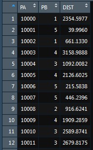
DistMin_Cent(Dist_mtx, "D", "DIST")

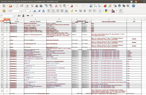
And then we can see the results of the process.

Update on Snowdoop, a MapReduce Alternative

Mad (Data) Scientist

In blog posts a few months ago, I proposed an alternative to MapReduce, e.g. to Hadoop, which I called “Snowdoop.” I pointed out that systems like Hadoop and Spark are very difficult to install and configure, are either too primitive (Hadoop)  or too abstract (Spark) to program, and above all, are SLOW. Spark is of course a great improvement on Hadoop, but still suffers from these problems to various extents.

The idea of Snowdoop is to

• retain the idea of Hadoop/Spark to work on top of distributed file systems (“move the computation to the data rather than vice versa”)
• work purely in R, using familiar constructs
• avoid using Java or any other external language for infrastructure
• sort data only if the application requires it

I originally proposed Snowdoop just as a concept, saying that I would slowly develop it into an actual package. I later put the beginnings of a…

View original post 601 more words

Installing R in Ubuntu

First of all, It’s possible to install R from the Ubuntu Software Center

But it’s so outdated, so some packages won’t work for maintenance issues.

To be able to install the current version you must modify the file sources.list

To do that, go to the terminal and type:

sudo nano /etc/apt/sources.list

And you should add the following line:

deb http://dirichlet.mat.puc.cl//bin/linux/ubuntu trusty/

That adress is because I’m on Chile, thus you have to replace it for the right mirror belonging to your country. To know that, just go to:

http://cran.r-project.org/mirrors.html

After you have modified the sources.list type the following:

sudo apt-get install r-base
sudo apt-get install r-base-dev

And now you have R ready to use it. Though, I recommend to use it along with RStudio.

Data Visualization cheatsheet, plus Spanish translations

RStudio Blog

We’ve added a new cheatsheet to our collection. Data Visualization with ggplot2 describes how to build a plot with ggplot2 and the grammar of graphics. You will find helpful reminders of how to use:

• geoms
• stats
• scales
• coordinate systems
• facets
• position adjustments
• legends, and
• themes

The cheatsheet also documents tips on zooming.

Download the cheatsheet here.

Bonus – Frans van Dunné of Innovate Online has provided Spanish translations of the Data Wrangling, R Markdown, Shiny, and Package Development cheatsheets. Download them at the bottom of the cheatsheet gallery.

View original post

RStudio v0.99 Preview: Code Completion

Great! This is very useful, it’s something we were waiting for.

RStudio Blog

We’re busy at work on the next version of RStudio (v0.99) and this week will be blogging about some of the noteworthy new features. If you want to try out any of the new features now you can do so by downloading the RStudio Preview Release.

The first feature to highlight is a fully revamped implementation of code completion for R. We’ve always supported a limited form of completion however (a) it only worked on objects in the global environment; and (b) it only worked when expressly requested via the tab key. As a result not nearly enough users discovered or benefitted from code completion. In this release code completion is much more comprehensive.

Smarter Completion Engine

Previously RStudio only completed variables that already existed in the global environment, now completion is done based on source code analysis so is provided even for objects that haven’t been fully evaluated:

Completions are also provided…

View original post 419 more words

Writing multiple csv files from a xlsx

What I used for this example is an open data about “Recycling places”, you can find it on the web page of Portal de datos Públicos.

The data, is an xlsx file

The file has 8 columns, one of them is town. So, now, the questions is:

How do I generate multiple files, one for each town?. The answer is simple: R

Why R? Because, you can automatize it. It avoid you to make different filters, and save the new file each time.

Let’s start:

To read the file, you can use the XLConnect package, and to split the data: the plyr package.

You can load the file with the function readWorksheet, but, as you can see, on the first row, six of the eight cells, are merged. So, when you load the file, that will disappear. Thus, we will read the file with headers and we’ll rename the columns with troubles; and then we will remove the row without data.

After that, we will use the d_ply function, which lets us to split the data. On this function, we put the field on which the split should be based. Then, we use the sdf function, which allows us to write the csv files; and as a final step, we extract the names from the field chosen, to paste them on the name of the new files.

library(XLConnect) #Functions to read excel
library(plyr) #Functions to split data

wb = loadWorkbook("Formato_Puntos_de_almacenamiento_Muni_consolidado.xlsx")
df = readWorksheet(wb, sheet = "Hoja1", header = TRUE)
colnames(df)[c(5, 6)] <- c("Este UTM", "Norte UTM")  #change col names
df2 <- df[-1,] #remove first row

d_ply(df2, .(Comuna),
      function(sdf) write.csv(sdf,
                              file=paste(sdf$Comuna[[1]],".csv",sep=""))) #write multiple csv